| If you find errors or omissions in this document, please don’t hesitate to submit an issue. |
Introduction
1. What is the TSX?
The TSX is the world’s first Threatened Species Index. It will do for Australia’s threatened species what the ASX does for Australia’s stock market. The TSX comprises a set of indices that provide reliable and robust measures of population trends across Australia’s threatened species. It will allow users to look at threatened species trends, for all of Australia and all species altogether, or for individual regions or groups, for example migratory birds. This will enable more coherent and transparent reporting of changes in biodiversity at national, state and regional levels. The index constitutes a multi-species composite index calculated from processed and quality controlled Australian threatened and near-threatened species time-series data based on the Living Planet Index (Collen et al. 2009) approach. The Living Planet Index method requires input on species population data repeatedly recorded for a species at a survey site carried out with the same monitoring method quantifying the same unit of measurement and aggregated from raw data into a yearly time series through time. This guide exemplifies how to use an automated processing workflow pipeline to streamline all processing steps required to convert raw species population data into consistent time series for the calculation of composite multi-species trends.
2. How to use this guide
This guide explains how to install and setup the TSX workflow, and then walks through the process of running the workflow on a provided sample dataset. It is highly recommended to run through this guide using the sample dataset to gain familiarity with the workflow before attempting to use it to process your own dataset. Many of the sample files provided will be useful starting points which you can modify to suit your particular dataset.
3. Workflow Concepts
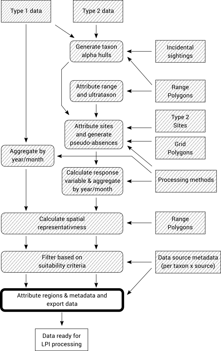
The TSX is produced using a workflow that begins with raw observation data collated into a relational database in a standardised way. These data are processed into time series that ultimately produce the index as well as diagnostics that provide additional context. The overall structure of the workflow is illustrated below.
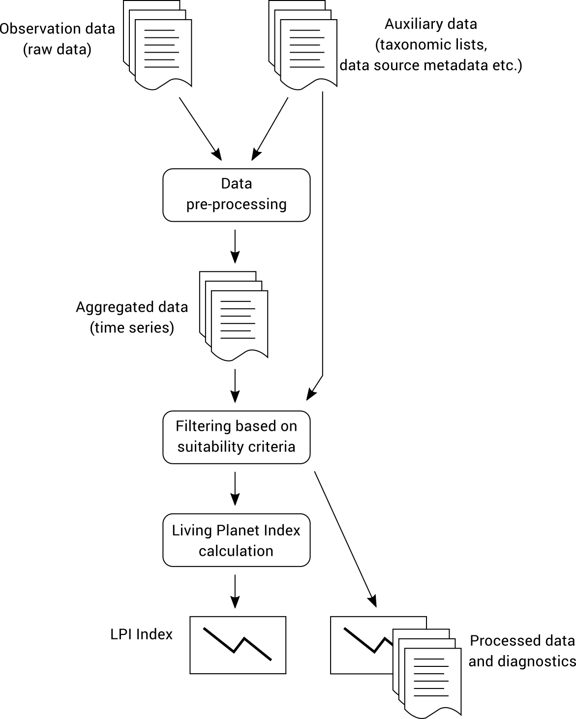
The observation data must be provided to the workflow in a specific format and is classified as either Type 1 or Type 2 data (see Data Classification). The workflow performs much more complex processing on Type 2 data than Type 1 data, so if your data meets the Type 1 requirements then running the workflow will be quicker and easier.
4. Architecture
The data import, pre-processing and filtering steps are performed using Python scripts that operate on a relational MySQL database. The last step of Living Planet Index calculation is performed using an R script, which operates on a CSV file that is produced by preceding steps of the workflow. This is illustrated below.
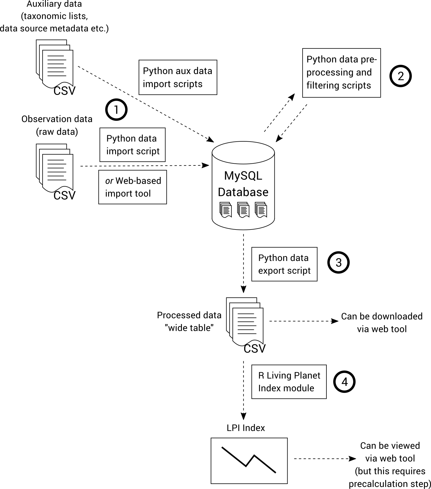
A web interface can be used to import data and view the generated indices, diagnostics and processed data. This is not an essential element of the workflow and is not covered in this guide.
Installation and Setup
5. System requirements
The TSX workflow can run on Windows, macOS or Linux. 8GB RAM and 4GB available storage space is recommended.
6. Installation methods
The workflow was primarily designed to run on Linux and macOS, and requires several prerequisite software packages to be installed. Performing the installation directly onto a Windows is possible, but is complicated and not recommended for most users.
We also supply a Docker Compose configuration that is pre-configured to run the TSX workflow.
6.1. Installation using Docker (recommended)
If you do not already have Docker installed on your machine, we recommend installing Docker Desktop via https://docs.docker.com/get-started/get-docker/. If you install Docker using a different method, you must ensure that Docker Compose is also installed. You can check this by attempting to run docker compose on the command line/terminal.
Download the TSX code from https://github.com/nesp-tsr3-1/tsx to your machine.
Using the command line/terminal, run the following command inside the folder containing the TSX code.
docker compose run --build --rm workflow_cliThe first time you run this command, Docker will need to download packages and build the necessary containers, which can take a few minutes. When the containers have been loaded, you will be presented with a command prompt which you can use to follow along with the rest of this guide. The command prompt looks like this:
TSX:/tsx#The first time you run the TSX Workflow container, you will need to initialise the database by running:
TSX:/tsx# mysql -u root -proot tsx < db/sql/create.sql
TSX:/tsx# mysql -u root -proot tsx < db/sql/init.sql
TSX:/tsx# mysql -u root -proot tsx < sample-data/seed.sql
Please note the following:
-
The folder containing the TSX code will be shared with the Docker container, so you can access any files that you place in the folder from the TSX Workflow command prompt.
-
When the workflow is running in Docker, you can access the MySQL database admin interface by going to http://localhost:8033/index.php?route=/database/structure&db=tsx
-
To completely reset the database and containers, run
docker compose --profile '*' down -v. Then start the TSX workflow container again and run the commands above to initialise the database again.
You can now proceed to Running the workflow.
6.2. Installation on Linux/macOS
6.2.1. Install Prerequisite software
The following instructions have been tested on Ubuntu Linux 18.04. If you are using a different Linux distribution you will need to adapt these commands for your system. If you are using macOS, we recommend using homebrew (https://brew.sh) to install dependencies.
Run the following commands to install prerequisite software:
sudo apt-get update
sudo apt-get install -y --no-install-recommends libgdal-dev r-base r-base-dev git build-essential libharfbuzz-dev libfribidi-dev  libfontconfig1-dev libgit2-dev libssl-dev  default-mysql-client libbz2-dev curl
Install uv by following the instructions at https://docs.astral.sh/uv/getting-started/installation/
6.2.2. Download TSX Workflow and Sample Data
Run the following command to download the TSX workflow into a folder named tsx
git clone https://github.com/nesp-tsr3-1/tsx.gitThen enter the tsx directory and run the following commands to install Python and R dependencies:
uv sync
Rscript -e 'renv::restore()'
6.2.3. Database Setup
Initialise the database by running:
sudo setup/setup-database.sh
sudo mysql tsx < sample-data/seed.sql
Understanding the database schema is not essential to following the steps in this guide, but is recommended if you want to gain an in-depth understanding of the processing.
6.2.4. Update Workflow Configuration File
Copy the sample configuration file from TSX_HOME\tsx.conf.example to TSX_HOME\tsx.conf.
cp tsx.conf.example tsx.conf6.3. Installation on Windows (advanced)
6.3.1. Install Prerequisite software
MySQL Community Edition 8
Download: https://dev.mysql.com/downloads/mysql/
Choose the ‘Developer Default’ Setup Type which includes MySQL Workbench - a graphical user interface to the database (not required to run the workflow but makes it easier to inspect the database). At the ‘Check Requirements’ installation menu click ‘next’. Follow the default installation settings unless indicated otherwise. Under ‘Accounts and Roles’ choose a password and make sure to remember it later on.
Anaconda
The rest of the required software can be installed using Anaconda. Anaconda enables you to conveniently download the correct versions of Python, R and libraries in one step, and avoids any conflicts with existing versions of these software that may already exist on your computer.
6.3.2. Download TSX Workflow and Sample Data
The latest version of the TSX workflow software can be downloaded at: https://github.com/nesp-tsr3-1/tsx/archive/master.zip .
Download and unzip into a directory of your choosing (or clone using Git if you prefer). To make it easier to follow this guide, rename the tsx-master directory to TSX_HOME. (Depending on how you unzip the file, you may end up with a tsx-master directory containing another tsx-master directory – it is the innermost directory that should be renamed.)
Now open Anaconda and use the 'Import Environment' function to import the conda-environment.yml file inside the TSX_HOME directory. Importing this environment will take some time as Anaconda downloads and installs the necessary software. Once the environment has been imported, click the 'play' icon next to the environment to open a Command Prompt which can be used to run the TSX workflow.
This guide will make extensive use of this Command Prompt. All commands assume that your current working directory is TSX_HOME, so the first command you will need to run is cd to change your working directory.
6.3.3. Database Setup
Start the MySQL command-line client and create a database called “tsx”. In this guide we will simply be accessing MySQL as the default “root” user. (Note that in a shared environment it is advised to create a separate user that has limited access to the tsx database only.)
mysql –u root
mysql> create database tsx;
mysql> quit;
Now run the following commands to populate the database structure and lookup tables.
mysql –u root tsx < db\sql\create.sql
mysql –u root tsx < db\sql\init.sql
mysql –u root tsx < sample-data\seed.sql
Understanding the database schema is not essential to following the steps in this guide, but is recommended if you want to gain an in-depth understanding of the processing.
6.3.4. Update Workflow Configuration File
Copy the sample configuration file from TSX_HOME\tsx.conf.example.windows to TSX_HOME\tsx.conf.
copy tsx.conf.example.windows tsx.confRunning the workflow
7. Data Import
The database and workflow tools are now configured and ready for auxiliary and observation data to be imported.
7.1. Taxonomic List
Before observation data can be imported, a taxonomic list must first be imported which identifies all valid taxa that will be processed by the workflow. A sample taxonomic list containing Australian birds can be found in sample-data/TaxonList.xlsx.
The Taxonomic list file format is a useful reference if you want to build your own taxonomic lists for use in the workflow.
Import the sample taxonomic list:
uv run python -m tsx.import_taxa sample-data/TaxonList.xlsxIf the import is successful, the command will complete without any output.
7.2. Import Type 1 data
Type 1 observation data may now be imported into the database. Some sample Type 1 data can be found in sample-data/type_1_sample.csv. Import this data, by running the following command:
uv run python -m tsx.importer --type 1 -c sample-data/type_1_sample.csvThe --type 1 part of the command tells the import script that you are importing Type 1 data. This is important because Type 1 data has different requirements and is stored in a separate database table compared to Type 2 data. The -c flag is short for “commit” and causes the imported data to be committed to the database; without this flag, the command only performs a “dry run” and does not modify the database. This feature is also present in most of the data processing scripts, and is a useful way to test whether the data/processing is valid without actually making any change to the database.
The import script will run a range of checks on the imported data, which will generate warnings and/or errors. Warnings are advisory, while errors will prevent the data from being imported until they are fixed. This helps to ensure data quality.
The Type 1 data is now imported into the t1_survey, t1_sighting and t1_site database tables and is ready for data processing. You may choose to skip the rest of this section, which deals with importing Type 2 data, and proceed directly to Data Pre-processing & Filtering.
7.3. Import Type 2 data
Type 2 data is imported in much the same way as Type 1 data. Sample Type 2 data can be found in sample-data/type_2_sample.csv. Import this data by running the following command:
uv run python -m tsx.importer --type 2 -c sample-data/type_2_sample.csvThis imports data into the t2_survey and t2_sighting tables.
7.4. Import Region Polygons
During data processing, all observations are matched to Interim Biogeographic Regionalisation subregions (SubIBRA regions). The Interim Biogeographic Regionalisation for Australia (IBRA), Version 7 classify Australia’s landscapes into 89 large geographically distinct bioregions based on common climate, geology, landform, native vegetation and species information. Within these, there are 419 subregions which are more localised and homogenous geomorphological units in each bioregion. Observations outside of SubIBRA regions are suppressed from the final output.
Import the SubIBRA regions into the database:
uv run python -m tsx.import_region sample-data/spatial/Regions-simplified.shp| Calling this command can take up to 20–30 minutes to process depending on you computer. |
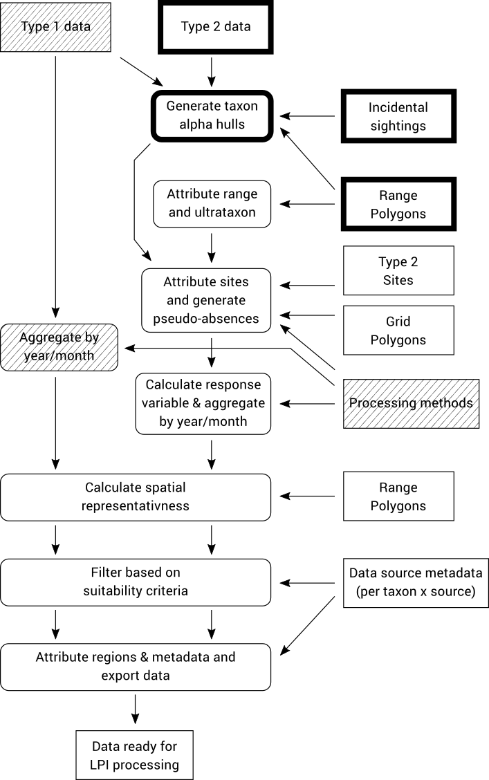
8. Data Pre-processing & Filtering
Now that the observation data has been imported into the database, it is ready to be processed and filtered into an aggregated form that is suitable for LPI (Living Planet Index) analysis.
The figure below illustrates the individual steps required to process Type 1 and 2 data. Each processing step is a separate Python script that needs to be run. It is possible to run all of the scripts in a single command, however it is often useful to be able to run the steps individually especially when tweaking processing parameters and inputs. Each command stores its output in the database, so all intermediate results in the processing pipeline can be inspected and analysed.
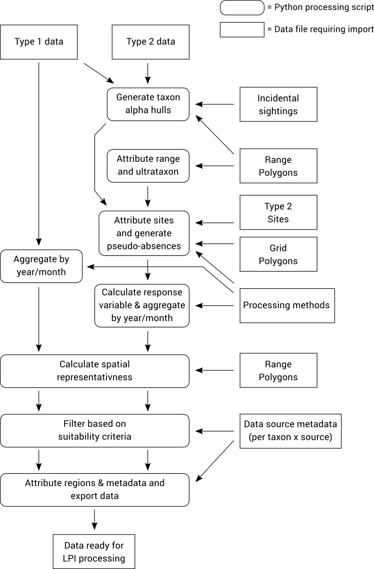
In the documentation below, all steps that specific to Type 2 data only are clearly marked and can be safely skipped if you only want to process Type 1 data.
8.1. Aggregate Type 1 data by year/month
Observation data is aggregated to monthly resolution by grouping all records with the same month, taxon, data source, site, method (search type) and units of measurement.
Each group of records is aggregated by calculating the average value, maximum value or reporting rate (proportion of records with a non-zero value) of the individual records. Which of these three aggregation methods are used for each grouping is determined by the “Processing methods” file which specifies which aggregation method should be used for each taxon/source/method/unit combination.
For further information, see Processing methods file format.
After monthly aggregation, the data is then aggregated to yearly by averaging the monthly aggregated values.
The sample processing methods file is available at sample-data/processing_methods.csv. Import this by running:
uv run python -m tsx.import_processing_method sample-data/processing_method.csvTo aggregate the Type 1 data by month and year, run the following command:
uv run python -m tsx.process -c t1_aggregationThis will aggregate the data and put the result into the aggregated_by_year and aggregated_by_month tables.
You may now choose to skip to Calculate spatial representativeness (Type 1 & 2 data) if you are not processing Type 2 data at this stage.
8.2. Generate taxon alpha hulls (Type 2 data only)
Type 2 data typically contains presence-only data, however the LPI analysis requires time series based on data that include absences (or true zeros indicating non-detections). To solve this problem we need to generate (pseudo-)absences for surveys where a taxon was not recorded but is known to be sometimes present at that location. In order to identify areas where the pseudo-absences should be allocated for a species, we first generate an alpha hull based on all known observations of the species. The alpha hulls are drawn from all Type 1 and 2 data, as well as an “Incidental sightings” file which contains observation data that did not meet the Type 1 or Type 2 criteria but is still useful for determining potential presences of a taxon.
After generating these alpha hulls at the species level they are trimmed down to ultrataxon polygons by intersecting with expert-curated polygons of known taxon ranges that are defined in an auxiliary “Range Polygons” input file.
There is a sample incidental sightings input file at sample-data/incidental_sightings.csv, which can be imported by running:
uv run python -m tsx.import_incidental sample-data/incidental_sightings.csvThere are sample range polygons at sample-data/spatial/species-range/, which can be imported by running:
uv run python -m tsx.import_range sample-data/spatial/species-range| Ignore the warning ‘Failed to auto identify EPSG: 7’ popping up while this processing step is running. |
The specifications for both the incidental sightings file and the species range polygons can be found in the Appendix.
After importing these files, you can then run the alpha hull processing script:
uv run python -m tsx.process -c alpha_hull| Calling this command may take a few minutes depending on your computer. |
This will perform the alpha hull calculations, intersect the result with the range polygons, and places the result into the taxon_presence_alpha_hull database table.
8.3. Aggregate Type 2 data by year/month
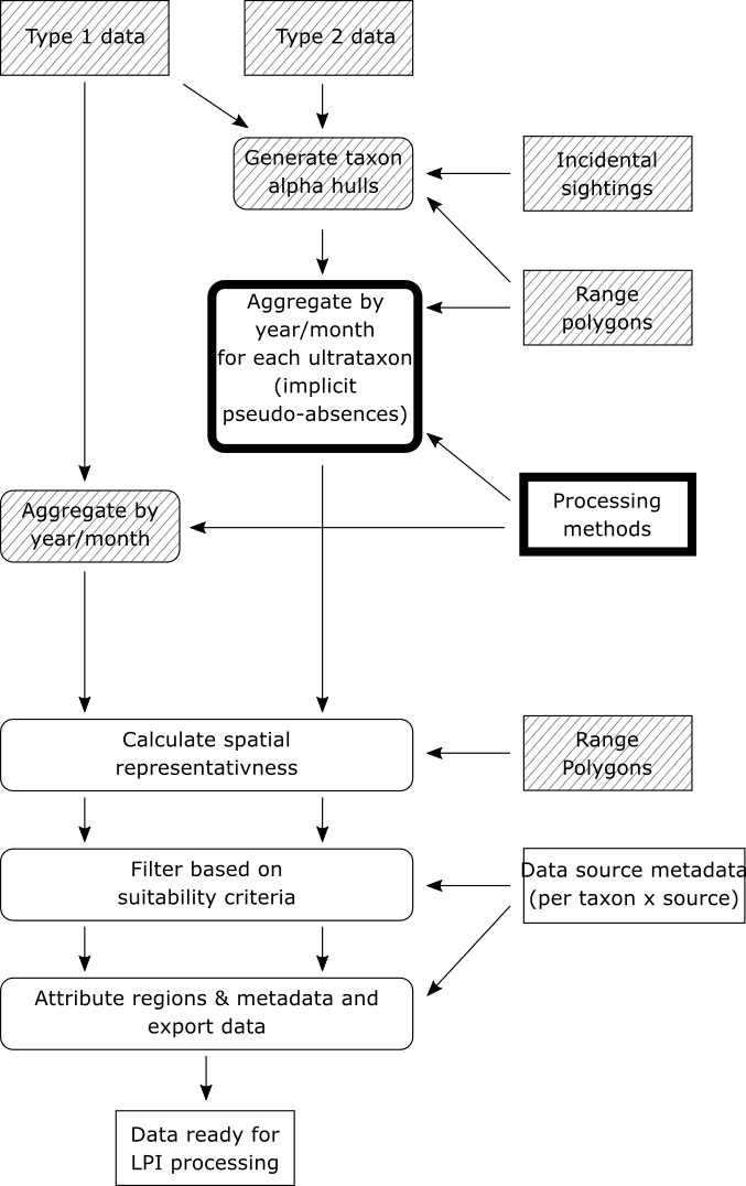
Now that alpha hulls have been calculated for each ultrataxon that we are interested in, we can proceed with aggregating the type 2 data.
This step of the workflow makes these assumptions about type 2 data:
-
Only occupancy (UnitID=1) and abundance (UnitID=2) units are supported; sightings with any other units are ignored.
-
All sightings with occupancy units (UnitID=1) are presences; i.e. there are no explicit absences with occupancy units. We refer to these as "presence-only" sightings.
-
All surveys are explicity associated with a site in the imported data file.
The workflow performs the following processing steps for each ultrataxon of interest:
-
A list is made of all sites associated with at least one survey that falls inside the ultrataxon’s alpha hull. In other words, a list is made of all sites where the ultrataxon is known to occur.
-
A list is made of all surveys in these sites. Note that each survey either contains a sighting record for the ultrataxon (a presence-only or abundance count) or it does not not (a pseudo-absence). Importantly, if the ultrataxon is a subspecies and a survey contains a sighting of its parent species, that sighting is considered to be sighting of the ultrataxon for the purposes of this workflow step.
-
These surveys are aggregated into monthly time series by grouping together records with the same year, month, site, search type and source, calculating the following values for each group:
-
The number of surveys (\$n_s\$)
-
The number of surveys with presence-only sightings of the current ultrataxon (\$n_p\$)
-
The number of surveys with abundance sightings of the ultrataxon (\$n_a\$)
-
The sum of all counts for abundance sightings of the ultrataxon (\$s\$)
-
The maximum count for abundance sightings of the ultrataxon (\$m\$)
-
-
These values are then used to calculate the following response variables of interest:
-
reporting rate: \$(n_p + n_a)/n_s\$
-
mean abundance: \$s/(n_s - n_p)\$
-
max abundance: \$m\$
-
-
All though all 3 response variables are calculated, only the response variables specified in the processing methods file are actually kept for further processing.
-
The monthly time series are then further aggregated to yearly time series by taking the average value of the response variable across all months in each year for which data exists.
Note that the mean abundance calculation includes pseudo-absences as zeroes, rather than simply being a mean of counts of sightings with abundance units.
The type 2 aggregation we have just described can be performed by running the following command
uv run python -m tsx.process -c t2_aggregationThis will aggregate the data and put the result into the aggregated_by_year and aggregated_by_month tables, alongside any existing aggregated type 1 data.
8.4. Calculate spatial representativeness (Type 1 & 2 data)
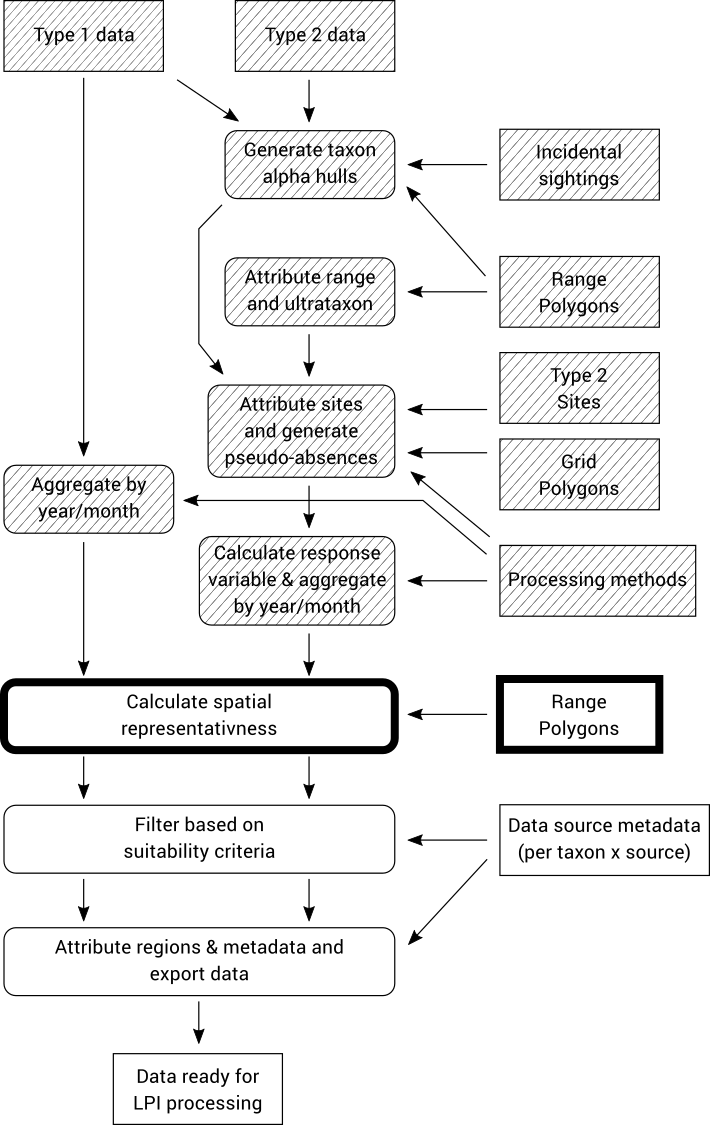
Spatial representativeness is a measure of how much of the known range of a taxon is covered by a given data source. It is calculated by generating an alpha hull based on the records for each taxon/source combination, and then measuring the proportion of the known species range that is covered by that alpha hull.
This step requires the range polygons file to be imported first. If you skipped to this section from the Type 1 data aggregation step, then you will need to import this now. A set of sample range polygons can be imported by running:
uv run python -m tsx.import_range sample-data/spatial/species-rangeThe spatial representativeness processing can now be run with this command:
uv run python -m tsx.process -c spatial_repThis will produce alpha hulls, intersect them with the taxon core range, and populate them into the taxon_source_alpha_hull database table. The area of the core range and the alpha hulls is also populated so that the spatial representativeness can be calculated from this.
Note that both Type 1 and Type 2 data (if imported and processed according to all the preceding steps) will be processed by this step.
8.5. Filter based on suitability criteria (Type 1 & 2 data)
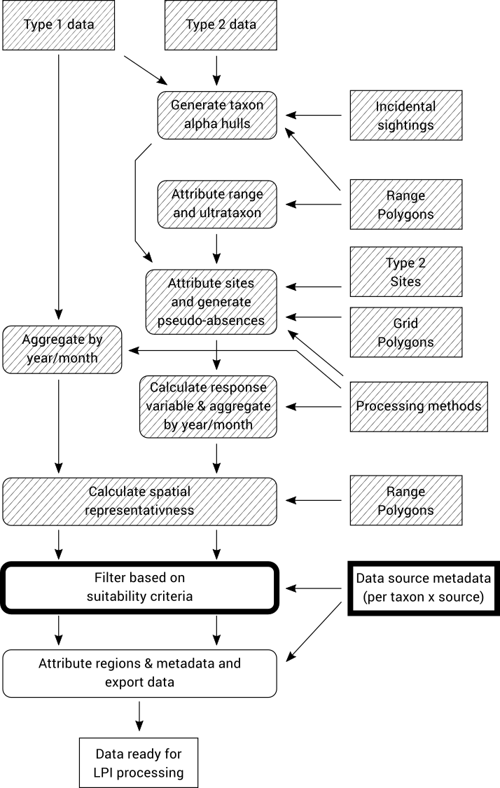
The final step before exporting the aggregated time series is to filter out time series that do not meet certain criteria.
The time series are not actually removed from the database in this step, instead a flag called include_in_analysis (found in the aggregated_by_year table) is updated to indicate whether or not the series should be exported in the subsequent step.
The filtering criteria applied at the time of writing are:
-
Time series are limited to min/max year as defined in config file (1950-2015)
-
Time series based on incidental surveys are excluded
-
Taxa are excluded if the most severe EBPC/IUCN/Australian classification is Least Concern, Extinct, or not listed.
-
Surveys outside of any SubIBRA region are excluded
-
All-zero time series are excluded
-
Data sources with certain data agreement, standardisation of method and consistency of monitoring values in the metadata are excluded
-
Time series with less than 4 data points are excluded
In order to calculate these filtering criteria, data source metadata must be imported (See Data sources file format).
Sample metadata can be imported by running:
uv run python -m tsx.import_data_source sample-data/data_source.csvThe time series can then be filtered by running:
uv run python -m tsx.process -c filter_time_series8.6. Attribute regions & metadata and export data (Type 1 & 2 data)
The data is now fully processed and ready for export into the “wide table” CSV format that the LPI analysis software requires.
To export the data, run:
uv run python -m tsx.process export_lpi --filterThis will place an output file into sample-data/export/lpi-filtered.csv.
This file is ready for LPI analysis!
It is also possible to export an unfiltered version:
uv run python -m tsx.process export_lpior a version aggregated by month instead of year:
uv run python -m tsx.process export_lpi --monthly8.7. Run it all at once
It is possible to run all the data pre-processing & filtering in a single command:
uv run python -m tsx.process -c allAfter which you must export the data again, e.g.:
uv run python -m tsx.process export_lpi --filterThis is useful when you import some updated input files and wish to re-run all the data processing again.
9. Living Planet Index Calculation
The Living Planet Index is used to generate the main final output of the TSX workflow.
The data pre-processing & filtering generates a CSV file in a format suitable for the Living Planet Index R package, rlpi.
To open RStudio and open an example script for generating the TSX output:
(cd r; rstudio lpi.R)After a short delay, RStudio should appear.
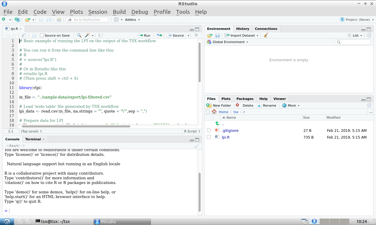
Press Shift+Ctrl+S to run the LPI. After running successfully, a plot should appear in the bottom left window (you may need to click on the 'Plots' tab):
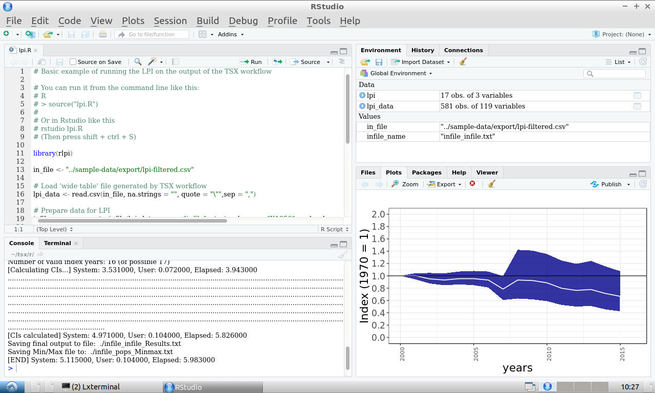
Congratulations! You have now run the entire TSX workflow.
9.1. LPI calculation via command line
Alternatively, you can run the LPI calculation directly on the command line:
(cd r; Rscript lpi.R)This will generate the result data in a file named infile_infile_Results.txt (inside the r subdirectory), but it will not display a plot. However, a plot will be generated in a file called Rplots.pdf.
To run the entire workflow, including the LPI calculation, run the following command:
uv run python -m tsx.process -c all && uv run python -m tsx.process export_lpi --filter && (cd r; Rscript lpi.R)Working with your own data
10. Starting afresh
Up to this point we have been working with sample data in order to gain familiarity with the TSX workflow. The purpose of this section is to explain how to run the workflow with your own input data.
If you have been working through the guide with the sample data, clear out all data from the database by running these two commands:
mysql tsx < db/sql/create.sql
mysql tsx < db/sql/init.sql
Now, work again through each step in the Running the workflow section, this time adapting each command for your particular use case. For every command that involves a file from the sample-data directory, you will need to evaluate whether the sample-data is appropriate for your use case, and if not, edit it or supply your own file as necessary. The Import File Formats section will be useful when working with these files.
| If you get stuck, you can get in touch by submitting an issue here. |
11. Accessing files in VirtualBox
If you have installed the TSX workflow using VirtualBox, then the entire workflow is running inside a virtual machine. This virtual machine saves you the hassle of installing and configuring all the different components of the TSX workflow, but it does have a drawback: you can’t access the files inside the virtual machine like the same way as ordinary files on your computer. This presents a problem when you want to provide your own files as inputs to the workflow, or edit the sample data using the usual methods.
Fortunately, however, there are a couple of ways to get around this limitation.
11.1. Accessing files via network sharing
The TSX virtual machine shares its files using network sharing so that you can access them in the same way that you would access files from another computer on your network. Don’t worry if your computer isn’t connected to an actual network, these steps should work regardless.
To access the TSX files, open File Explorer and go to Network. If you see an error message ("Network discovery is turned off…."), you’ll need to turn on Network discovery to see devices on the network that are sharing files. To turn it on, select the Network discovery is turned off banner, then select Turn on network discovery and file sharing.
You may see a TSX icon appear immediately, but if not, try typing \\TSX into the location bar near the top of the window and pressing enter.
You should now be able to browse and edit files in the TSX virtual machine. If not, try the following: - If you have only just started the virtual machine, try waiting for a few minutes before retrying the steps above. - Report an issue at https://github.com/nesp-tsr3-1/tsx/issues - Try the alternative method, Accessing files via SFTP
11.2. Accessing files via SFTP
An alternative to network sharing is to access the files over SFTP.
First you will need to download an SFTP program, such as WinSCP. (Download WinSCP)
Start WinSCP, and in the Login Dialog, enter the following details:
-
File protocol:
SFTP -
Host name:
localhost -
Port number:
1322 -
User name:
tsx -
Password:
tsx
Then click Login to connect.
You should now be able to browse the TSX files. Unlike the networking sharing method, you can’t edit the files directly on the virtual machine. Instead you will have to edit the files in a folder on your computer’s hard drive, and download and upload files from the virtual machine as necessary.
Appendix A: Import File Formats
A.1. Taxonomic list file format
File format: Excel Spreadsheet (xlsx)
Sample file: TaxonList.xlsx
Column |
Notes |
TaxonID |
Required, alphanumeric, unique |
UltrataxonID |
Boolean: “u” = is an ultrataxon, blank = is not an ultrataxon |
SpNo |
Numeric species identifier (must be the same for all subspecies of a given species, and must be part of the TaxonID) |
Taxon name |
Text, common name of taxon |
Taxon scientific name |
Text |
Family common name |
Text |
Family scientific name |
Text |
Order |
Text |
Population |
Text, e.g. Endemic, Australian, Vagrant, Introduced |
AustralianStatus |
Text, optional, one of:
|
EPBCStatus |
As above |
IUCNStatus |
As above |
BirdGroup |
Text, e.g. Terrestrial, Wetland |
BirdSubGroup |
Text, e.g. Heathland, Tropical savanna woodland |
NationalPriorityTaxa |
Boolean (1 = true, 0 = false) |
SuppressSpatialRep |
Boolean (1 = true, 0 = false), optional (defaults to false) If true, spatial representativeness will not be calculated for this taxon |
A.2. Processing methods file format
File format: CSV
Sample file: processing_methods.csv
Column |
Notes |
taxon_id |
Alphanumeric, must match taxonomic list |
unit_id |
Numeric, must match IDs in the |
source_id |
Numeric, must match IDs in the |
source_description |
Text, must match description in the |
search_type_id |
Numeric, must match IDs in the |
search_type_description |
Text, must match description in the |
data_type |
Numeric, 1 or 2 – determines whether this row applies to type 1 or type 2 data |
response_variable_type_id |
Numeric
|
positional_accuracy_threshold_in_m |
Numeric, optional Any data with positional accuracy greater than this threshold will be excluded from processing |
A.3. Incidental sightings file format
File format: CSV
Sample file: incidental_sightings.csv
Column |
Notes |
SpNo |
Numeric species identifier as per taxonomic list |
Latitude |
Decimal degrees latitude (WGS84 or GDA94) |
Longitude |
Decimal degrees longitude (WGS84 or GDA94) |
A.4. Range polygons file format
File format: Shapefile
Sample files: spatial/species-range/*
Column |
Notes |
SPNO |
Numeric species identifier as per taxonomic list |
TAXONID |
Taxon ID as per taxonomic list (this should be an ultrataxon), or for hybrid zones an ID of the form u385a.c which denotes a hybrid zone of subspecies u385a and u385c |
RNGE |
Numeric
|
A.5. SubIBRA Region Polygons file format
Citation: Australian Government Department of the Environment and Energy, and State Territory land management agencies. 2012. IBRA version 7. Australian Government Department of the Environment and Energy and State/Territory land management agencies, Australia.
Format: Shapefile
Sample file: spatial/Regions.shp
Column |
Notes |
RegName |
Text, name of region |
StateName |
Text, name of state/territory |
A.6. Data sources file format
Format: CSV
Sample file: data_sources.csv
Column |
Notes |
SourceID |
Numeric, must match id in source database table |
TaxonID |
Alphanumeric, must match id in taxon database table |
DataAgreement |
Numeric
|
ObjectiveOfMonitoring |
Numeric
|
AbsencesRecorded |
Numeric
|
StandardisationOfMethodEffort |
Numeric
|
ConsistencyOfMonitoring |
Numeric - 1 = Highly imbalanced because different sites are surveyed in different sampling periods and sites are not surveyed consistently through time (highly biased). - 2 = Imbalanced because new sites are surveyed with time but monitoring of older sites is not maintained. Imbalanced survey design may result in spurious trends - 3 = Imbalanced because new sites are added to existing ones monitored consistency through time - 4 = Balanced; all (>90%) sites surveyed in each year sampled |
StartYear |
Numeric, optional, records before this year will be omitted from filtered output |
EndYear |
Numeric, optional, records after this year will be omitted from filtered output |
NotInIndex |
Boolean (1 = all records will be omitted from filtered output, 0 = records will be included in filtered output, subject to other filtering rules) |
SuppressAggregatedData |
Boolean (0 = no, 1 = yes), does not affect processing but is simply copied to the final output to indicate that aggregated data from this data source should not be published. |
Authors |
Used to generate citations for this data source |
Provider |
Used to generate citations for this data source |
12. Accessing files in Docker
To access your own files when running the workflow via Docker, place them inside the data folder which is automatically created in the same folder as the 'docker-compose.yml' file when you first run the workflow. Files in this folder are accessible from the Docker workflow command prompt. For example if you placed a file called my-surveys.csv into this folder, then you could import them in the Docker workflow command prompt by running:
uv run python -m tsx.importer --type 1 -c my-surveys.csv ---
Appendix B: Data Classification
B.1. Type 1 data
Type 1 data must satisfy the following requirements:
-
Species are defined to the ultrataxon level (i.e. terminal taxonomic unit of species such as species or a subspecies, hereafter referred to as ‘taxa’
-
The survey methods (e.g. capture-mark-recapture surveys) are clearly defined
-
The unit of measurement (e.g. number of individuals, nests, traps counted) is defined
-
Data is recorded to the temporal scale of at least a year
-
Spatial data for have defined accuracy of pre-defined (fixed) sites where the taxon was monitored through time
-
Consistent survey methods and monitoring effort are used to monitor the taxon
-
Non-detections of taxa (i.e. absence or 0 counts) are recorded and identifiable within the data
B.2. Type 2 data
Type 2 data must satisfy the following requirements:
-
Taxon is defined at least to species level
-
Survey methods are clearly defined
-
The unit of measurement is defined
-
Consistent survey methods and monitoring effort are used to monitor the taxon through time
-
Data are recorded to the temporal scale of at least a year
-
Non-detections of taxa are not required, i.e. presence-only data are allowed
-
Spatial coordinates are available for all sighting data points